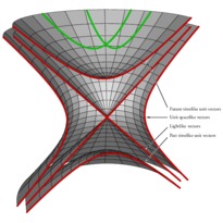
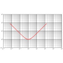
En cliquant sur une imagette, vous accéderez au source et à l'image. En cliquant sur cette dernière, vous ouvrirez le fichier PDF associé.
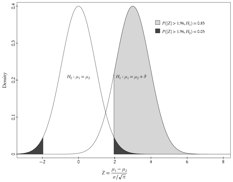
/* -*-ePiX-*- */
#include "epix.h"
using namespace ePiX;

double f(double x) { return 0.4*exp(-x*x/sqrt(M_PI)); }
double g(double x) { return f(x-3); }

double PAD_X=0.4, PAD_Y=0.01;
const double legend_x=4.5, dx=0.25;
const double legend_y=0.35, dy=0.15*0.075;

int main() {
  bounding_box(P(-3-PAD_X,-PAD_Y),P(8+PAD_X,0.4+PAD_Y));
  unitlength("1in");
  picture(5.5,4);

  begin();
  degrees();
  grid(1,1);

  fill();
  gray(0.2);
  shadeplot(g, 1.96, x_max, 120);
  rect(P(legend_x-dx, legend_y), P(legend_x, legend_y+dy));


  gray(0.8);
  shadeplot(f, x_min, -1.96, 20);
  shadeplot(f, 1.96, 4, 40);
  rect(P(legend_x-dx, legend_y-2*dy), P(legend_x, legend_y-dy));


  fill(false);
  plot(f, x_min, x_max, 240);
  plot(g, x_min, x_max, 240);


  h_axis(P(-2,y_min), P(8, y_min), 5);
  v_axis(P(x_min, 0), P(x_min, 0.4), 4);

  std::cout << "\n\\begin{scriptsize}";
  label(P(legend_x, legend_y), P(4,2), "$P(|Z|>1.96, H_1) = 0.85$", r);
  label(P(legend_x, legend_y-2*dy), P(4,2), "$P(|Z|>1.96, H_0) = 0.05$", r);

  label(P(0, 0.2), P(0,2), "$H_0$: $\\mu_1=\\mu_2$", t);
  label(P(2, 0.2), P(2,2), "$H_1$: $\\mu_1=\\mu_2+\\delta$", tr);
  std::cout << "\n\\end{scriptsize}";

  std::cout << "\n\\begin{footnotesize}";
  h_axis_labels(P(-2,y_min), P(8, y_min), 5, P(0,-4), b);

  label(P(2, y_min), P(0,-18),
	"$Z=\\displaystyle\\frac{\\mu_1-\\mu_2}{\\sigma/\\sqrt{\\pi}}$", b);

  label_angle(90);

  v_axis_labels(P(x_min, 0), P(x_min, 0.4), 4, P(-4,0), l);

  label(P(x_min, 0.2), P(-18,0), "Density", l);

  std::cout << "\n\\end{footnotesize}";
  end();
}