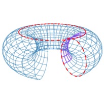
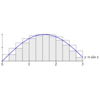
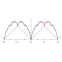
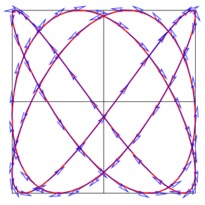
En cliquant sur une imagette, vous accéderez au source et à l'image. En cliquant sur cette dernière, vous ouvrirez le fichier PDF associé.
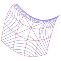
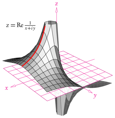
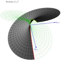
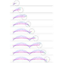
/* -*-ePiX-*- */
#include "epix.h"
using namespace ePiX;
const int M=8;
double MAX=1.5, Bd=2;
P F(double x, double y) // fake pole
{ return P(x, y, x/(0.01+x*x+y*y)); }
P pt1(-MAX,-MAX), pt2(MAX, MAX);

int main()
{
  bounding_box(P(-Bd,-Bd), P(Bd,Bd));
  unitlength("1in");
  picture(2.5,2.5);
  offset(2.25,-0.5);

  begin();
  domain R(pt1, pt2, mesh(2*M,2*M), mesh(6*M,6*M));
  label(P(x_min, y_max), P(2,-2), "$z=\\mathrm{Re}\\,\\frac{1}{x+iy}$", br);
  viewpoint(6,8,5);

  clip(); clip_box(P(-Bd,-Bd,-Bd), P(Bd,Bd,0)); fill(); surface(F, R); // bottom half
  gray(0); rect(pt1, pt2);  fill(false);
  pen(0.15); rgb(0.75,0.75,0.75); plot(F, R); plain();  // simulate transparency

  clip(false); magenta(); grid(pt1, pt2, M, M); // axes
  arrow(P(-Bd,0,0), P(Bd,0,0));  label(P(Bd,0), P(-4,-2), "$x$", l);
  arrow(P(0,-Bd,0), P(0,Bd,0));  label(P(0,Bd), P( 2,-2), "$y$", br);
  arrow(P(0, 0, 0), P(0,0,2.5)); label(P(0,0,2.5), P(0,4), "$z$", t);

  clip(); clip_box(P(-Bd,-Bd,0), P(Bd,Bd,Bd)); fill(); surface(F, R); // top half
  fill(false); pen(1.5); red(); plot(F, R.resize1(0.5,MAX).slice2(0));
  end();
}